Inhomogeneous Poisson process & case study
In this article I introduce the notion of inhomogeneous Poisson process and show a case study how it can be applied. This generalizes and expands the ideas developed in the articles about counting events and waiting times.
To recap, we have previously derived the (homogeneous) Poisson point process as follows: When we have a sequence of I.I.D. exponentially distributed random variables, which we interpret as waiting time between some events, then the number of events that occur within a fixed time interval has Poisson distribution. The exponential distribution itself can be derived from the memoryless assumption.
Now when we want to model a practical problem, we should look critically at these assumptions. I have discussed previously when the memorylessness assumption may or may not be appropriate. Here we will take a closer look at the situation when the I.I.D. assumption does not hold.
Introduction
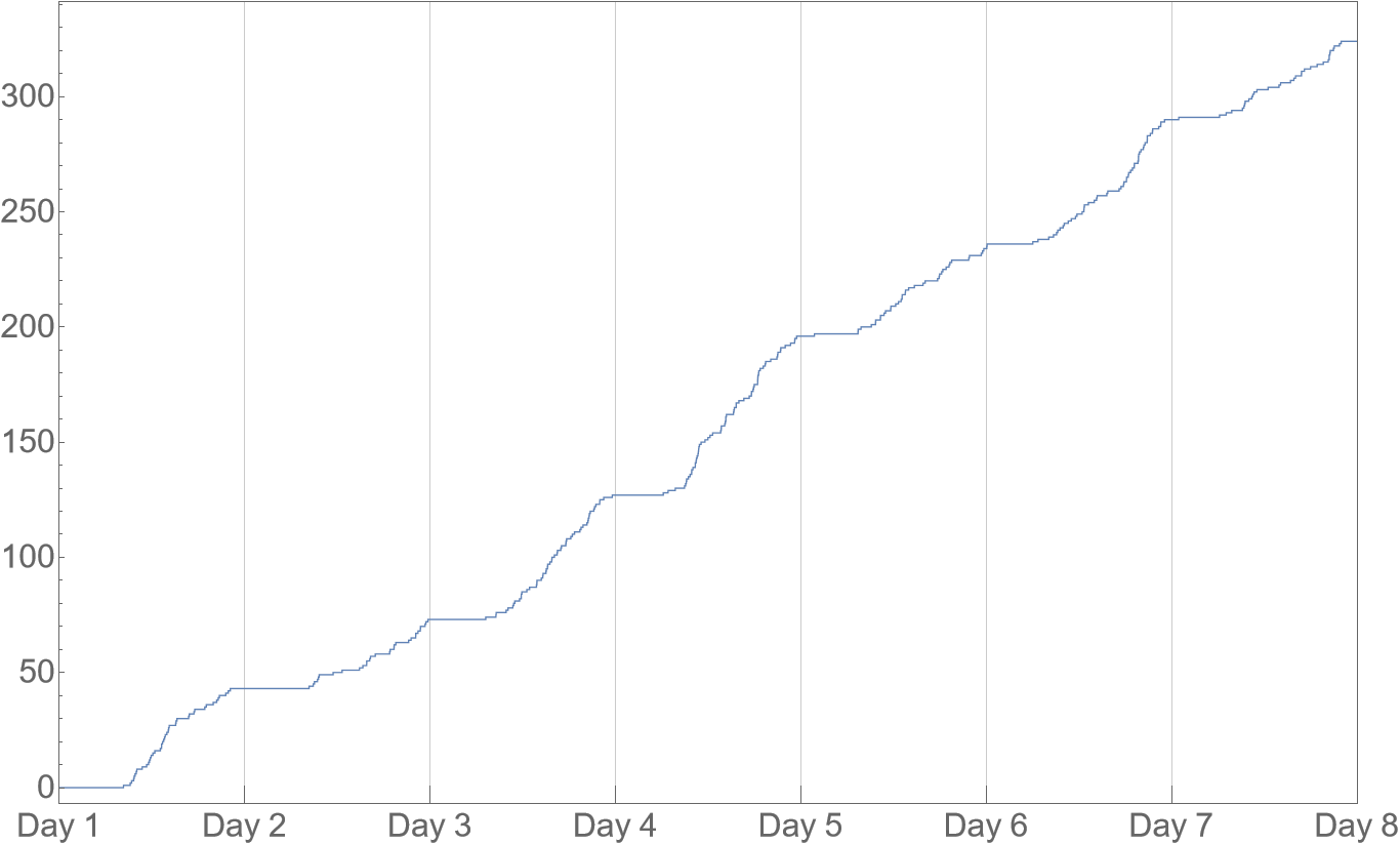
Let’s first see some data as an illustration. The following plot shows cumulative purchase counts over a week.
We can see that almost all the purchases happen between around 6AM and 12PM. This means the waiting times for next purchase are clearly a lot longer during the night than during the day, and thus they can’t be identically distributed. We may still use exponential distribution, assuming that memorylessness holds at least short-term, but the rate will not be a constant. Symbolically, $\lambda \in \mathbb{R}^+$ no longer holds, and instead we have $\lambda: (0, T) \to \mathbb{R}^+$, where $(0, T)$ is a temporal interval we’re interested in.
This is an inhomogeneous Poisson process – the rate of the exponential waiting times is non-constant in time. There are some technical requirements for well-behavedness of $\lambda(t)$, but for more precise and formal definition, along with some basic properties I refer to [1] and there is something on wikipedia too. For what I want to show here, an intuitive understanding should be enough: We have a process that is only “locally Poisson”. The key property here is that the number of events within an interval $(T_0, T_1)$ has Poisson distribution with rate $\int_{T_0}^{T_1} \lambda(t) \mathrm{d} t$. Remember that the rate is also the expectation value, which is useful for prediction making.
Parameter estimation
From the statistical perspective, how do we fit this $\lambda(t)$ from data parametrically? We first need to assume the function $\lambda(t\,|\,\mathbf{\theta})$ is given by a certain formula, where we want to find the parameters $\mathbf{\theta}$. Choice of this formula can be seen as specifications of further assumptions about the system and that should usually follow some exploratory analysis of the data.
As usual with parameter learning, we use maximum likelihood estimation. But what is the likelihood function here? We should note that one sample is not a single event occurrence $t_i$ (since their differences are not identically distributed), but rather, the interval $(0, T)$ with the entire realization $\mathbf{t} = (t_1, …, t_n)$ where each $t_i \in I$. Fortunately, even one realization may be enough to reasonably learn, if there are enough event records compared to the number of parameters. The log-likelihood can be shown[1],[2] to be:
\[\ell(\mathbf{t}\,|\,\mathbf{\theta}) = \sum_{i=1}^n \log \lambda(t_i\,|\,\mathbf{\theta}) - \int_0^T \lambda(s\,|\,\mathbf{\theta}) \mathrm{d}s\]Intuitively, the sum accounts for the events that have occurred and the integral accounts for the events that did not occur, but could have. For more complicated functions, the integral will likely not have an analytic solution and we the need to resort to numerical methods to evaluate the likelihood or use sampling algorithms to find the parameters.
Modelling – case study
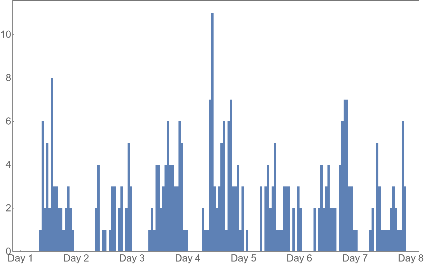
Briefly looking at the previous plot, I have mentioned that there is some sort of periodicity visible. It may be even clearer when we look at the aggregated hourly counts.
A simple three-parameter elementary function for this case may look like:
\[\lambda(t\,|\,\alpha,\varphi,\sigma) = \alpha \cdot \exp^{\sigma}(\cos(t-\varphi)-1)\]Where $\sigma \in \mathbb{R}^+$ controls the “width” of the bump, $\alpha \in \mathbb{R}^+$ is the amplitude and $\varphi \in (-\pi,\pi)$ is the phase shift. Of course, we assume the data have been scaled so that the length of one day is $2\pi$. The exponential is here to guarantee rate positivity and is somewhat convenient to work with, the $-1$ in the $\cos$ isn’t even necessary, but makes $\alpha$ directly interpretable as peak height. This function is inspired by the von Mises distribution density for circular data. I am not arguing this is the best choice here, just that it’s a choice that we can reasonably expect to give better predictive results for this particular data than just using the homogeneous process model.
The definite integral here, assuming additionally that $T = 2\pi k, k \in \mathbb{N}$ (i.e. we are analyzing a whole number $k$ of days), does not depend on $\varphi$ and can be expressed in terms of the modified Bessel function of the first kind (proof):
\[\int_0^T \lambda(s\,|\,\alpha,\varphi,\sigma) \mathrm{d}s = T \cdot \alpha \cdot e^{-\sigma} \cdot I_0(\sigma)\]although this is not elementary, it’s established enough to be implemented in various libraries where you can also do optimization. And just to be clear, the sum in the log-likelihood in this case simplifies (trivially) to:
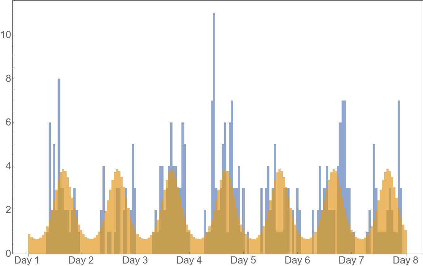
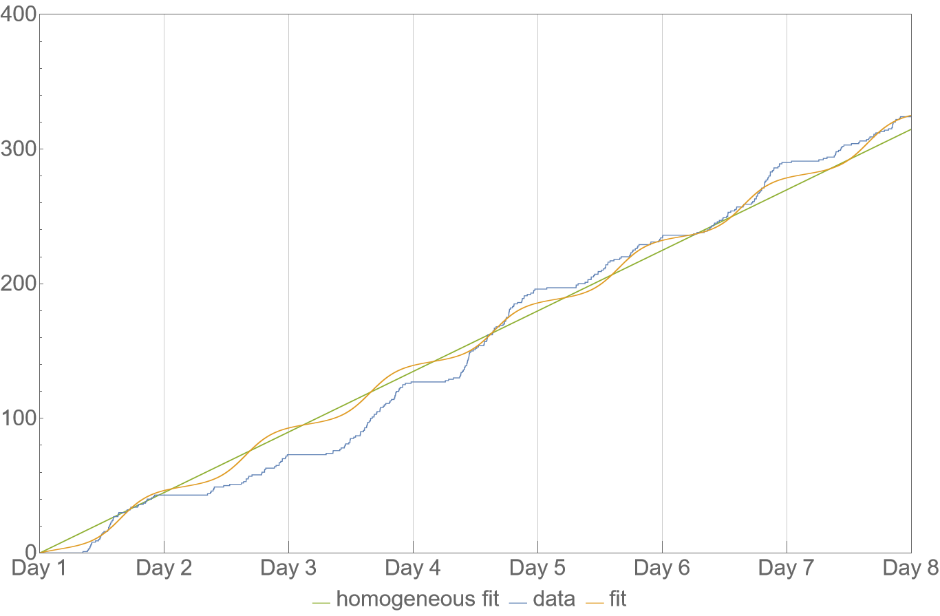
\[\sum_{i=1}^n \log \lambda(t_i\,|\,\alpha,\varphi,\sigma) = n(\log(\alpha)-\sigma) + \sigma \sum_{i=1}^n \cos(t_i-\varphi)\]Now we can find the parameter values using our favorite numerical optimizer (see Appendix). The results are shown on the following plots. Visually, it seems not great not terrible? But I think this is decent considering I’m only using three parameters. Given the relatively low amount of data, it’d be easy to overfit with more.
The chosen function doesn’t allow to easily capture the fact that there is almost nothing during night, but on the other hand it does seem pretty robust during the day. Perhaps a rectangular wave would be good too. But the trigonometric functions are nice in the sense that they are the golden standard in Fourier analysis where we can use them to express arbitrary periodicities, which provides a natural way to extend the ideas presented here.
Next read: Generalized linear models
References
- Anna Vedyushenko, Non-homogeneous Poisson process - estimation and simulation, Master thesis
- Mathematics StackExchange, Log likelihood of a realization of a Poisson process?
Appendix – Code
Optimization in Wolfram Script is short code:
1
2
3
4
5
6
7
8
9
T = 2*k*Pi;
loglike = (
  sigma*Total[Cos[data - phi]]
  + (Log[alpha]-sigma)*Length[data]
  - alpha*T*Exp[-sigma]*BesselI[0, sigma]
);
constraints = sigma > 0 && alpha > 0 && -Pi < phi <= Pi;
NMaximize[{loglike, constraints}, {alpha, sigma, phi}]
But I like STAN probabilistic modelling, even though the code is more verbose, it can be more naturally integrated with Bayesian techniques.
1
2
3
4
5
6
7
8
9
10
11
12
13
14
15
16
17
18
19
20
21
22
23
24
25
26
27
functions {
  real my_process_lpdf(data vector t, data real T, real alpha, real phi, real sigma) {
    return sigma*sum(cos(t-phi))
         + (log(alpha)-sigma)*size(t)
         - alpha*T*exp(-sigma)*modified_bessel_first_kind(0, sigma);
  }
}

data {
  int<lower=0> N;
  int<lower=0> k;
  vector<lower=0,upper=T>[N] t;
}

transformed data {
  real T = 2*k*pi();
}

parameters {
  real<lower=0> alpha;
  real<lower=0> sigma;
  real<lower=-pi(),upper=pi()> phi;
}

model {
    t ~ my_process(T, alpha, phi, sigma);
}


