From linear regression to GLMs – theory and examples

In this article, I dig a bit under the surface of the theory around good’ol linear regression and explain how it can be extended to generalized linear models and why GLMs may be useful on some examples.

One important case where linear regression fails when modelling time series is when the data are positive integers close to zero (e.g. daily counts of purchases of a low-selling product.) This is because there are certain assumptions encoded in the model, that we often justify with some handwavy reference to the central limit theorem. But in this case it may easily lead to poor results: For small counts, the distinction between normal and a discrete counting distribution will be significant. (See the article about counting events for a more detailed discussion.)

Generalized linear models (GLMs) max fix this and similar issues by allowing other kinds of data distributions while keeping a lot of the desirable and familiar properties of linear regression.

Linear regression

Everybody knows good-old linear regression. But it’s a good point where to start with the topic, so let’s recap a bit. First, let’s study the relation of linear regression and ordinary least squares (OLS).

Gauss–Markov theorem

OLS are the most basic and most common method to make a linear fit and is usually justified by referring to the Gauss–Markov theorem which says that ordinary least squares are the best linear unbiased estimator under certain conditions.

In particular: We call an estimator unbiased when $\mathrm{E}[\hat{\beta}] = \beta$. We say it’s best in the sense of statistical efficiency, i.e. we want to minimize $\mathrm{Var}[\hat{\beta}]$.

Have

\[\begin{equation}\label{eq:linreg}y = X\beta + \varepsilon,\end{equation}\]

where $y,\varepsilon \in \mathbb{R}^n, \beta \in \mathbb{R}^k, X \in \mathbb{R}^{n\times k}$ and individual $\varepsilon_i$ are understood as random variables. Since $y$ depends on $\varepsilon$, can also be analyzed as a random variable and so can be any estimate $\hat{\beta}$ which depends on $y$. Assume the error terms $\varepsilon$ have zero mean, i.e. $\mathrm{E}[\varepsilon_i] = 0$, and all have the same variance (homoscedasticity) and are uncorrelated i.e. $\mathrm{Cov}[e_i, e_j] = \sigma^2 \delta_{ij}$ where $\sigma \in \mathbb{R}^+$ (here using the Kronecker delta symbol). Gauss-Markov theorem says that under these conditions, the OLS estimator, given by

\[\hat{\beta} = \arg\min_{\beta} \lVert X\beta - y \rVert_2^2 = \arg\min_{\beta} \sum_i | X_i \beta - y_i|^2 = \left(X^T X\right)^{-1} X^T y\]

is the best estimator among those which are unbiased.

This is quite powerful, because it doesn’t specify which distribution $\varepsilon$ has, only that it needs to have certain properties.

But what if we decided we want to maximize efficiency, perhaps even at the cost of having the estimator biased?

MLE for linear regression

To do MLE, we need a distribution. So let’s now specify what distribution the error terms $\varepsilon$ have. The most common choice of model is:

\[\begin{equation}\label{eq:normalerr} \varepsilon_i \sim \mathrm{Normal}(0, \; \sigma^2), \end{equation}\]

where $\sigma \in \mathbb{R}^+$ is constant. The assumptions of the Gauss–Markov theorem are satisfied. Coincidentally, it can be shown that the maximum likelihood estimation of $\beta$ is in this case again OLS.

But what if the errors have a different distribution? For example Laplace.

\[\varepsilon_i \sim \mathrm{Laplace}\left(0, \; \theta'\right)\]

Now the assumptions of the Gauss–Markov theorem are still satisfied, but the MLE is the least absolute deviations (LAD), in other words, we use the $l^1$ norm instead of $l^2$:

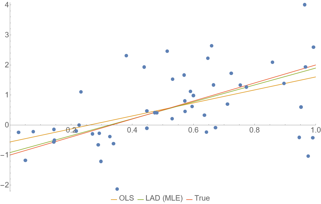
\[\hat{\beta} = \arg\min_{\beta}\mathscr{l}(X,y|\beta) = \arg\min_{\beta} \lVert X\beta - y \rVert_1 = \arg\min_{\beta} \sum_i | X_i \beta - y_i|\]

Under usual circumstances, MLE estimates are statistically efficient, at least asymptotically. The following plot shows some synthetic data with Laplace distributed noise around the red line. The fit obtained from the (biased) MLE is in this case closer to the true generating line on most of the interval, than the unbiased OLS suggested by Gauss–Markov. To understand how often this happens, we’d need to analyze the bias–efficiency relation exactly in more detail, but I’m not doing that now. In general though, the difference is not very big, so in practical cases, consider whether this is worth the headache.

(Fun fact: If you want general $l^p$ norm, there is Generalized normal distribution. The limit case for $p \to \infty$ with the max norm corresponds to uniform distribution of errors.)

The takeaway here should be that if we aren’t satisfied with the handwavy reference to CLT, and we have a reason to believe the distribution of the data is other than normal, we can likely do better than OLS. Note that the Laplace distribution has heavier tail than normal, so LAD may be practical to use in the presence of outliers in the data as it’s more robust.

Generalized linear models

With the Laplace distribution instead of normal, we have touched the idea of using different noise distribution. Generalized linear models (GLM) take this one step further. First, consider the case with the normal distributed noise and make a few simple observations. Putting together $\eqref{eq:linreg}$ and $\eqref{eq:normalerr}$ can be written as:

\[\begin{equation}\label{eq:normalerr2} y \sim \mathrm{Normal}\left(X\beta, \; \sigma^2 \mathbf{1}\right) \end{equation}\]

and thus also trivially:

\[\mathrm{E}\left[y|X\right] = X\beta.\]

Now we want to generalize this to another distribution $\mathcal{D}\left(\theta, \theta’\right), \theta \in \Theta$. Basically we want to plug $X\beta$ into the distributions parameter which represents the mean value. A lot of distributions don’t have that and may not even allow negative values though, so we allow a reparametrizazion function $g: \Theta \to \mathbb{R}$ (invertible), called the link function and require:

\[\begin{equation}\label{eq:link1}y \sim \mathcal{D}\left(g^{-1}\left(X\beta\right), \; \theta'\right) \end{equation}\]

and

\[\begin{equation}\label{eq:link2} \mathrm{E}\left[y|X\right] = g^{-1}(X\beta). \end{equation}\]

(Don’t ask me why the inverse link is used in most places, it’s just a weird convention.) The choice of the link function is kind of arbitrary as long as its domain is the parameter space, but it does have an effect on how the model performs and how it should be interpreted. The treatment of the extra parameters $\theta’$ may vary. In the simplest cases they don’t exist or are set to a fixed known value. Otherwise, they may be treated as nuisance parameters and approached with profile likelihood (or marginalization in a Bayesian setting) or they may be fully fledged parameters estimated jointly with $\beta$, which then may make the estimation more difficult. These details may be implementation–specific in software.

When the distribution $\mathcal{D}$ is from the exponential family and $\eqref{eq:link1},\eqref{eq:link2}$ hold, there are available good-performance algorithms to compute the likelihood and to maximize it. which are implemented in numerous libraries.

A famous instance of a GLM is the logistic regression, where $\mathcal{D}(\theta), \theta \in (0,1)$ is the Bernoulli distribution, and we use the logit function as the link. So in terms of $\eqref{eq:link1}$, logistic regression can be characterized as the probabilistic model:

\[y \sim \mathrm{Bernoulli}\left(\frac{1}{1+e^{-X\beta}}\right)\]

When $y$ is binary, the Bernoulli distribution is the only option, but as I mentioned, we can choose a different link function. In this case, quantile function of normal distribution is another possible option which is also sometimes used as the link function, leading to the somewhat less popular probit model.

For discrete counts data $y$, we can use distributions like Poisson, binomial, geometric or negative binomial which are all in the exponential family and are thus GLM–compatible.

GLM - example with data

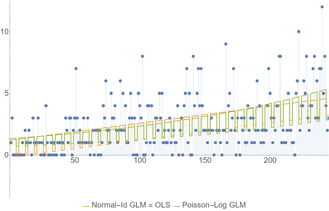
The following plot shows a comparison of using the OLS (a.k.a. Normal-Identity GLM) versus Poisson GLM with log link on some counts of daily purchases data. Just to be super clear, the models I’m comparing here are $\eqref{eq:normalerr2}$ and:

\[y \sim \mathrm{Poisson}\left(e^{X\beta}\right)\]

Although it may not be immediately obvious, the data do have some sort of trend growth and weekly periodicity, in particular there are less sales on weekends which is something modelling here.

For both GLMs, there are the same three features: intercept, the time (horizontal axis), and a boolean indicator for weekends.

A glaring (qualitative) issue with the OLS is that it can (and does near the axes origin) go into negative numbers, which would need to be solved using some ad-hoc technique like clipping which feels pretty arbitrary. The Poisson-log model will always produce a positive expectation value. But it has its own (quantitative) issue, here it’s simplicity is at the cost of an exponential trend growth which is unrealistic to use for extrapolation beyond very short term. (This can be avoided by not using time as a feature directly, but when we do, the log link must be interpreted as saying “we’re expecting exponential growth”). In this example, the Poisson-log model has better quality metrics like BIC, RMSE, MAE, but only marginally.

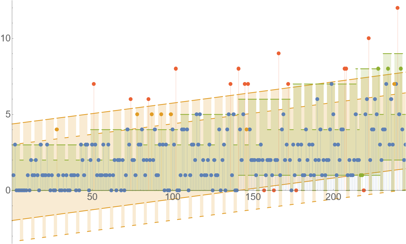
Where the qualitative difference between the models becomes more obvious is when we look at the prediction intervals for $y$. The following plot shows the prediction intervals in which 90% of the most likely outcomes will be (exactly 90% for OLS, at least 90% for Poisson GLM due to its discrete nature, inclusive on the boundary.) Quantitatively, the bounds for the Poisson GLM are mostly tighter (despite covering greater probability), which is desirable.

Suppose a business customer asks you, how many items is he going to sell tomorrow. Do you think he better likes the answer “between 0 and 3” or “between minus 1.9 and 4.33”?

How are the intervals computed?

This is something that was a bit skipped over in my statistical data analysis class at university, so I needed to learn that later on. Again I want to explain how this works for vanilla linear regression $\eqref{eq:normalerr2}$ and then, how that extends to GLMs. There are two intervals (or bands of their boundaries) that we usually may be interested in: The confidence interval of the fit and the wider prediction interval, illustrated on the following plot which fits an OLS on some data with normally distributed error.

Since $\hat{\beta}$ is a random variable, the expectation of the model $X \hat{\beta}$ is also random. Using the fact that MLE is $\hat{\beta} = \left(X^T X\right)^{-1} X^T y$ together with a little bit of algebra exercise, we can obtain:

\[\begin{equation}\label{eq:beta_estimate} \hat{\beta} \sim \mathrm{Normal}\left(\beta, \; \sigma^2 \left(X^T X\right)^{-1}\right) \end{equation}\]

Now the confidence interval of the fit asks “How far is $X \hat{\beta}$ from $X \beta$ within a given confidence level?” On the plot, this is the inner region in which the red line falls with 90% certainty. Knowing the distribution of $\hat{\beta}$ makes this straightforward to compute using standard techniques. The theory around standard error elaborates on this.

The prediction interval asks “What is the range of a future observed value $\hat{y} = y|X,x$ with a given confidence level?” Here $X$ is the past observed data matrix and $x \in \mathbb{R}^k$ is a new vector of features for which we’re making a prediction. To answer this we will identify the distribution of $\hat{y} \in \mathbb{R}$. In this case, we have:

\[y|x,\hat{\beta},\hat{\sigma} \sim \mathrm{Normal}(x^T\hat{\beta},\; \hat{\sigma}^2)\]

where we need to additionally specify that the MLE of $\hat{\sigma}^2$, which is given by the usual population variance formula:

\[\hat{\sigma}^2 = \frac{1}{n}\left(y-X\hat{\beta}\right)^T\left(y-X\hat{\beta}\right)\]

has the $\chi^2$ distribution variant:

\[\begin{equation}\label{eq:sigma_estimate} \hat{\sigma}^2 \sim \mathrm{Scaled–Inverse–}\chi^2(n-k, \; \sigma^2) \end{equation}\]

(Side note: $\hat{\sigma}$ is biased, but it’s more efficient than the unbiased sample variance formula with $n-1$ in denominator. This again illustrates that MLE prefers efficient estimates over unbiased.) Anyway, to obtain the distribution of $\hat{y}$ we need to marginalize out both random variables $\hat{\beta},\hat{\sigma}$. This is the same as the predictive posterior distribution in Bayesian statistics where we interpret $\eqref{eq:beta_estimate},\eqref{eq:sigma_estimate}$ as priors. It is a bit more tedious calculation, but it can be done somewhat routinely to obtain that $\hat{y}$ has the t-distribution (shifted and scaled):

\[\begin{equation}\label{eq:y_predictive} \hat{y} \sim t_{n-k} \left(x^T\beta, \; \sigma^2 \frac{n}{n-k}\left(1 + x^T\left(X^T X\right)^{-1} x\right)\right) \end{equation}\]

where the parameters are expectation and variance. So when we want precise prediction bands, we can just use this. However, it may be a bit awkward to work with and it doesn’t generalize well to other cases. So asymptotics to the rescue! With growing number $n$ of samples in $X \in \mathbb{R}^{n\times k}$, we are kinda back where we started and get back to the original normal distribution in the sense that:

\[\lim_{n\to\infty}\hat{y} \sim \mathrm{Normal}(x^T \beta, \; \sigma^2)\]

or we could basically just write:

\[\hat{y} \approx y\]

This result should be intuitive: When we have enough data, there is little uncertainty about the coefficients $\hat{\beta}$ and thus this uncertainty doesn’t affect the prediction interval much; only the natural variance of $y$ does. It is also why in the plot, the prediction interval seems flat, even though it isn’t exactly (since the covariance in $\eqref{eq:y_predictive}$ depends on the position on the horizontal axis).

In general, for GAMs, there isn’t an explicit formula like $\eqref{eq:y_predictive}$ but the asymptotics are analogous and we get:

\[\lim_{n\to\infty} \hat{y} \sim \mathcal{D}\left(g^{-1}\left(x^T\beta\right), \; \theta'\right)\]

So for a confidence level $\gamma \in (0, 1)$, the approximate prediction interval is the smallest set $C$ such that

\[\int_C p_{\mathcal{D}}\left(y\;|\;g^{-1}\left(x^T\beta\right),\; \theta'\right) \, \mathrm{d}y \le \gamma\]

and analogically a sum for discrete distribution. Obviously, in practice, we must substitute the estimated values in place of $\beta, \theta$. This is how I constructed the prediction intervals for the Poisson–log GLM. Note that for multimodal $\mathcal{D}$, the set $C$ may not be an interval, but rather a disjoint set of intervals, but idk about any case where that would happen in modelling practice.

If we don’t want to use the asymptotic approximation, we must often resort to numerical methods.
A cool trick is to set some (non-informative) Bayesian priors over $\beta,\theta’$ and use MCMC style algorithms to compute posteriors of $\hat{y},\hat{\beta},\hat{\theta’}$ which can serve to analyze their uncertainty and determine the desired intervals.